| |
Introduction
Despite being prolific models, feed-forward neural networks have been ubiquitously
criticized for having a low degree of comprehensibility. A neural network
could be performing a task it was trained for perfectly, but to its users it
remains a black-box. What has it learned about the data it was trained on? Is
it generalizing in a consistent manner? For what inputs is the network untrustworthy?
These are questions we would like answers to. Different approaches have
been put to this problem such as Rule-Extraction, Contribution Analysis
and Network Inversion. In our approach we try to generate exact representations
of a network's function by analyzing the principles of its underlying
computation. Only by analyzing networks exactly can we learn their real strengths
and pitfalls: When they will generalize well, the relationship between
size and complexity, the relationship between dimensionality and complexity, when
will learning succeed and fail, etc.
In this page we present an
algorithm tthat extracts exact representations from feed-forward threshold neural networks
in the form of polytopic decision regions. We demonstrate its use on different
networks, and show what this extracted representation can tell us about
a network's function. We then use the underlying principles that the algorithm
is based on to calculate network and algorithmic complexity bounds as well as
raise questions about learning in neural networks.
|
| |
Algorithm Principals
The algorithm extracts polytopic decision regions from multi-layer multi-output
feed-forward threshold activation function networks.
The algorithm
is based on a few observations on how these neural networks compute:
- Networks are deterministic, output is a direct function of input.
- The location where an output unit switches values is a Decision Boundary.
This corresponds to a change in the output units' partial sum, which in turn
corresponds to a change in the output of one or more hidden units.
- The locations of change are at the intersections of the first hidden layer's units'
hyperplanes.
-
The network divides up the input space into polytopic
Decision Regions whos verticies are at the intersections of the hidden unit
hyperplanes.
|
| |
Algorithm Logic
The Decision Intersection Boundary Algorithm (DIBA) receives as inputs the weights
of a three layer feed forward network and the bounds of the input space. Its output
consists of the vertex pairs, or line segment edges that describe the decision
regions in input space. The algorithm consists of two parts, a part which
generates all the possible vertices and connecting line segments, and a part that
evaluates whether these basic elements form the boundaries of decision regions.
- The generative part performs a recursion over the intersections
of the hidden unit hyperplanes. This is achieved by incrementally projecting
hyperplanes onto each other.
- A boundary in an n dimensional input
space demarcates the location of an output value transition. For an intersection
of hyperplanes to be a boundary we seek that all hyperplanes making up the
intersection have at least one face that acts as a boundary in its vicinity. The
same boundary test is used for vertices and edges.
|
| |
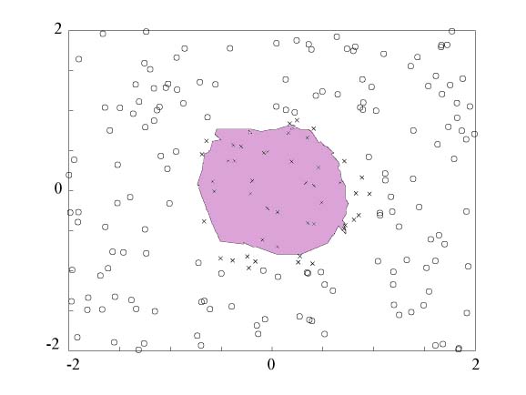
Circle Network
Using back-propagation, an 80 hidden unit sigmoidal network was trained to classify
points inside and outside of a circle of radius 1 around the origin. Treating
the activation functions as threshold, the DIBA algorithm was used to generate
the immediate figure showing the network's representation of the learnt
circle-- a decision region composed of the hidden unit line boundaries. The decision region fully describes
what the network is doing. That is, all points inside the
decision region will generate a network output of 1, and all the points outside the decision region
will generate a network output of 0. We can see that
the network did a pretty good job of encapsulating a circle-like decision regions, but we can also
see where the learned circle deviates from an actual circle and how
some of the training points were misclassified.
|
| |
 |
 |
| |
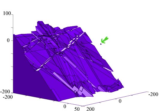
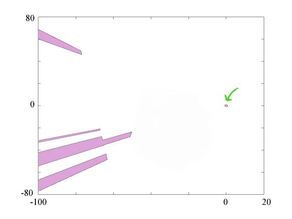
By zooming out from the area in the immediate vicinity of the origin we can see the
network's performance or generalization ability, in areas of the input space
that it was not explicitly trained for. In the figure we see some artifacts, decision
regions at a distance of at least 50 units from the decision region at the origin. This implies
a network misclassification if that part of the input space was of interest.
|
| |
 |
| |
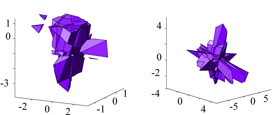
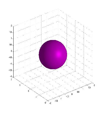
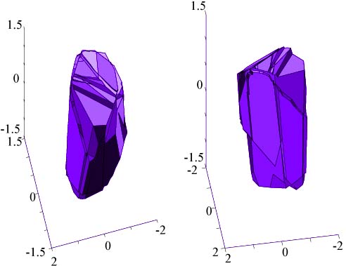
Sphere Network
A 100 hidden unit network was trained to differentiate between points inside
and outside of a sphere centered at the origin. The figure below illustrates
the network's sphere-like decision region from two angles. The figure below
shows the same artifact phenomena as in the circle network above-- the miniature sphere
appears amid a backdrop of an ominous cliff face decision region.
|
| |
 |
| |
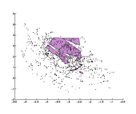
Vowel Recognition Network
Two neural networks were trained on vowel data available at the CMU repository.
This data consists of 10 log-area parameters of the reflection coefficients
of 11 different steady-state vowel sounds. Our interest in this example was to
gauge the effect of using input spaces of different dimensionality. Whether adding dimensions will
improve the generalization of the network. Both networks
were trained to recognize the vowel with the had sound contrasted with another 10
vowel sounds.
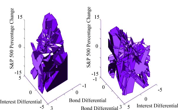
The first network received as input the first two coefficients.
After training, it achieved a better than 86% success rate on the training
data. The following figure illustrates its decision regions. In the input
region of [3.2,2.3]X[0.7,1.2] we see that many disparate decision regions are
used to secure a perfect classification.
|
| |
 |
| |
The second network received the first four coefficients as inputs. It achieved a
success rate of over 91% on the training data. It also achieved perfect classification
in the same input region. However it doesn't seem to have partitioned the
space. There is only one decision region in this area. If we slice this polytope
using four hyperplanes bisecting each of its dimensions, we only get 10 sub
polytopes, suggesting a small degree of concavity (less than the 16 we would
expect for a perfectly convex shape). In addition these sub-decision regions are
mostly delimited in the third and fourth dimension with the first two dimensions
ignored (span the whole space). Therefore, it appears that the network makes
use of these added dimensions to form a more regular decision region in that
difficult portion of the input space.
|
| |
Algorithm and Network Complexity
The Decision Intersection Boundary Algorithm's complexity stems from its transversal
of the hyperplane arrangement in the first layer of hidden units. As
such, that part of its complexity is equivalent to similar algorithms, such as
arrangement construction [Edelsbrunner 87], which are exponential in the input dimension.
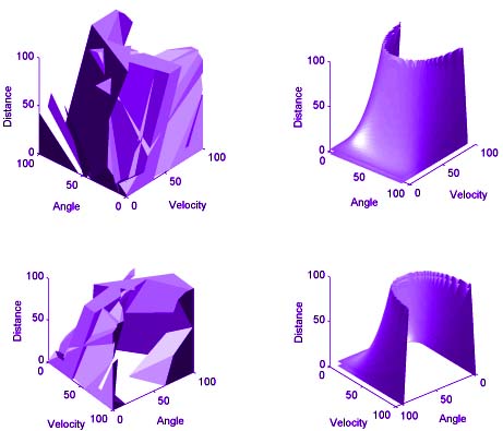
Do
we really need to examine every vertex though? Perhaps the network
can only use a small number of decision regions, or it is limited with respect
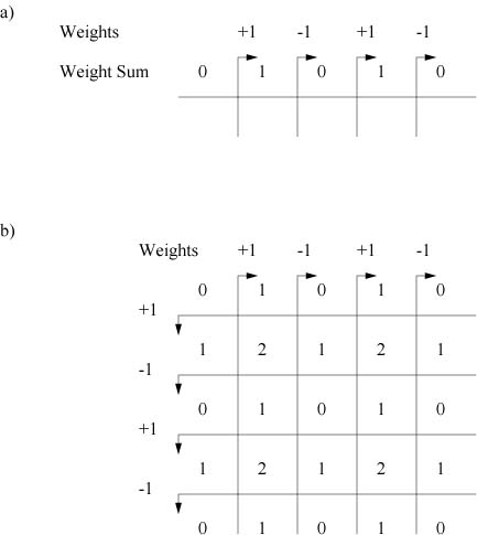
to the complexity of the decision regions. The following figure demonstrates that
a network is capable of exponential complexity by an inductive construction
of a network with an exponential number of decision regions, where each decision
region has an exponential number of vertices. The figure shows the inductive
step from one dimension to two dimensions. The zeros represent decision regions
(line in 1-D, squares in 2-D).
|
| |
 |
| |
Generalization and Learning
Generalization is the ability of the network to correctly classify points in
the input space that it was not explicitly trained for. In a semi-parametric
model like a neural network, generalization is the ability to describe the correct
output for groups of points without explicitly accounting for each point individually.
Thus, the model must employ some underlying mechanisms to classify
a large number of points from a smaller set of parameters.
In our feed-forward
neural network model we can characterize the possible forms of generalization
with two mechanisms. The first is by proximity: nearby points in the
same decision region are classified the same way. The second is by face sharing:
the same hidden unit hyperplane is used as a border face in either multiple decision
regions or multiple times in a decision region.
Given these two
mechanisms, how well do learning algorithms exploit them? It is intuitive that
learning algorithms which pull borders (Hyperplanes in this case) towards similar
output points and away from different output points, should be geared for
proximity generalization by forming decision regions. However face sharing is
more combinatorial in nature, and might not be as amenable to continuous deformation
of parameters as found in many algorithms.
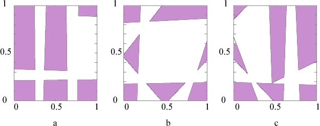
To illustrate this
point a group of 8 hidden unit neural networks were trained on the decision regions
illustrated in the 2-D complexity figure. One thousand data points were taken
as a training sample. Two hundred different networks were tested. Each was
initialized with random weights between -2 and 2, and trained for 300 online epochs
of backpropagation with momentum. Of the 200 networks none managed to learn
the desired 9 decision regions. The network with the best performance generated
6 decision regions (left figure) out of an initial two. However, in examining
its output unit's weights, we see that only one weight changed sign, the weight
initially closest to zero, indicating a predisposition to this configuration
in the initial conditions. The other figures are the decision regions of the more
successful networks.
|
| |
 |
| |
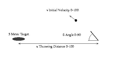
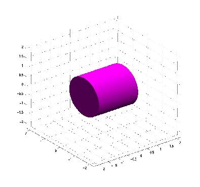
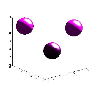
Network Learning Animations
If we can visualize the decision regions of a neural network, as is the case for networks with two or three inputs,
then we can visualize these networks as they learn-- watching how their decision regions are modified with iterations
of the learning algorithm. The following three movies are of networks trying to learn the decision region indicated by their
respective picture. That is, a network trying to learn a sphere, a cylinder and three separate spherical decision regions.
Each frame consists of the network's decision regions juxtaposed with a Hinton diagram of the network's weights.
The blue cloumn has the output unit's weights, while the gray rows are the hidden unit weights.
These movies are examples of relatively successful learning using backprop with momentum. Their successes are not the
norm, and more frequently than not learning will result in inappropriate or non-existant decision regions. Note, even
though we are interpreting the activation functions as threshold for the algorithm, backprop is treating them as sigmoids.
The implications of this are outlined in the tech-report.
|

 Movies of Learning
 Download Tech-Report
 Download the Software!